Introduction
The STILT results viewer is used to view footprint maps and simulated CO2 and CH4 concentration time series, calculated using the STILT calculation service. You will have to log in through ATMO-ACCESS to use either service through an ORCID, eduGAIN, or ENVRI community log-in.
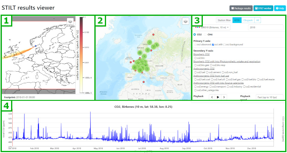
The results viewer consists of four sections, as shown in the screenshot below: 1) the footprint map; 2) the station selection map; 3) the configuration options panel; and 4) the tracer concentration time series graph.
Step 1: Select the station
First, select the station you would like to view results for. Use the station filter, at the top of the configuration options, to select which stations you would like to view – ICOS stations, Obspack stations, or All stations, which includes model results from user-defined locations. The station can be selected by either using the drop-down menu or by clicking on it on the station selection map, in the centre.
Step 2: Select the year
The drop-down menu lists those years for which STILT simulation results are available. If observational data are available for comparison, this is indicated in the drop-down list as well (e.g., "2021 (+ ObsPack 100 m)"). The European ObsPack collection includes the latest ICOS release of CO2 and CH4 data in addition to the ICOS near real time data.
After the selection of station and year, the footprints and CO2 or CH4 time series will be loaded.
Step 3: Select tracer: CO2 or CH4
Click on the radio button to the left of the tracer name to switch between CO2 and CH4, selecting which tracer will be used for the concentration time series graph and component display. The footprints are the same for both tracers.
Step 4: Select components of CO2 or CH4
By default, the STILT-simulated concentration time series (blue line) is shown and,if available, the observed CO2 or CH4 concentration time series (black line) is included as well. The values of the concentration time series are shown on the left-hand side (primary) y-axis.
In the model simulations the contributions from different fluxes can easily be separated. These contributions can be viewed separately, with their values appearing on the right-hand side (secondary) y-axis.
For CO2 the following contributions can be viewed separately:
- Contributions from natural fluxes co2.bio, split into:
- co2.bio.gee uptake of CO2 by photosynthesis
- co2.bio.resp release of CO2 by respiration
- Contributions from anthropogenic emissions, split into:
- fuel-type specific contributions:
- co2.fuel: co2.fuel.coal, co2.fuel.oil, co2.fuel.gas, co2.fuel.bio, co2.fuel.waste from burning of coal, oil, gas, biofuel, and waste
- co2.cement from cement production
- co2.non_fuel from other processes not related to fuel burning
- or emissions from different source categories:
- co2.energy includes energy production and refineries
- co2.industry includes industrial processes and manufacturing
- co2.transport includes road transportation, railways, shipping, and aviation
- co2.residential is residential heating
- co2.other_categories includes fuel exploitation and agricultural waste burning
- fuel-type specific contributions:
- Contributions from sources and sinks outside the model domain co2.background
For CH4 the following contributions can be viewed separately:
- Contributions from anthropogenic emissions ch4.anthropogenic, split into:
- ch4.agriculture includes enteric fermentation and manure management
- ch4.waste includes landfills and waste water management
- ch4.energy includes energy production, refineries and transmission
- ch4.other_categories includes transport, industrial processes, and residential heating
- Contributions from natural fluxes ch4.natural, split into:
- ch4.weltands includes emissions from peatlands and inundated soils
- ch4.soil_uptake is uptake in dry mineral soils
- ch4.wildfire is biomass burning emissions
- ch4.other_natural includes emissions from lakes, ocean, and wet mineral soils
- Contributions from sources and sinks outside the model domain ch4.background
Step 5: Animate the footprints
By default, the footprint for the central time step of the time series is displayed on the leftmost map. In the Playback area, below the options, you can use the controls to view the footprint at different time points. You can step through time using the arrows (‹ and ›) or play a continuous animation of the footprint by clicking the Play (▶) button.
Footprint display configuration:
- Change the timestep for which to display a footprint by clicking and dragging the red line, marking the current time step, to the left or right.
- Zoom in on the time axis to display selected range of the time series by clicking on a point on the graph and dragging left or right and then releasing. Double click anywhere on the graph to reset the zoom level.
- Zoom in on the concentration axis by clicking on a point on the graph and dragging up or down and then releasing. Double click anywhere on the graph to reset the zoom axis.
- Zoom in on the footprint map by using the +/- controls in the upper left corner of the footprint map or using the scroll wheel. Move the map view by clicking and dragging.
- Show or hide the station symbol and/or country borders on the footprint map by clicking on the "layers" icon in the upper right corner of the footprint map. Enable or disable options by clicking on the options.